CGAN笔记总结第二弹~

一、复习GAN

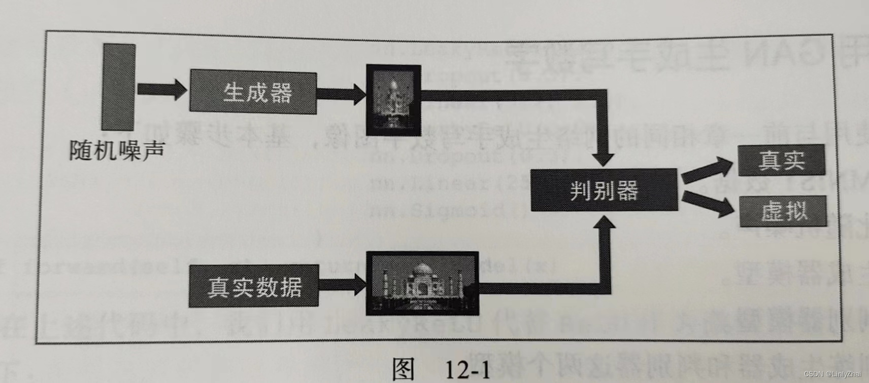
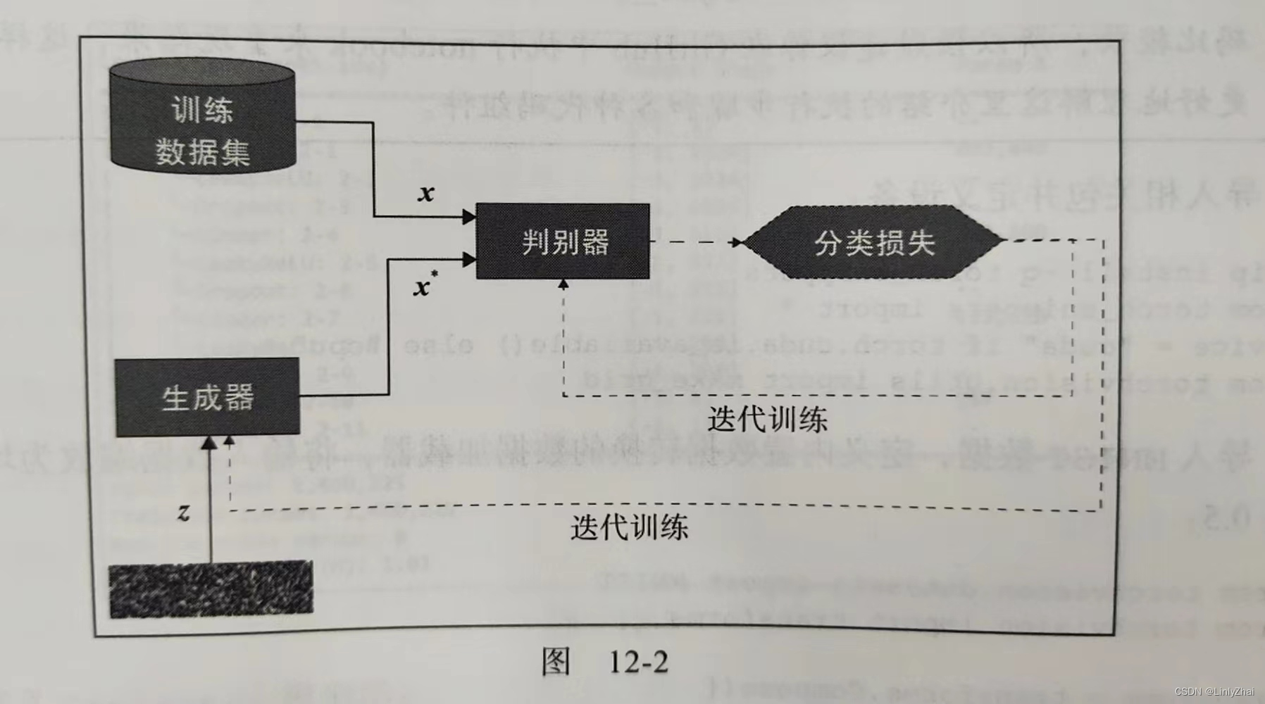
生成式对抗网络（Generative Adversarial Networks）是让两个神经网络进行博弈进行学习。基础结构包含生成器和判别器。生成器的目标是生成与真实图片相似的图片，以假乱真，尽可能地让判别器判断生成的图片是真实的。判别器的目标是能够区分真实图片和生成图片。生成器和判别器通过巧妙地设计损失函数，而结合在一起，在相互对抗中不断调整各自的参数，使得判别器难以判断生成器生成的图片是否真实，从而达到欺骗人眼的效果。

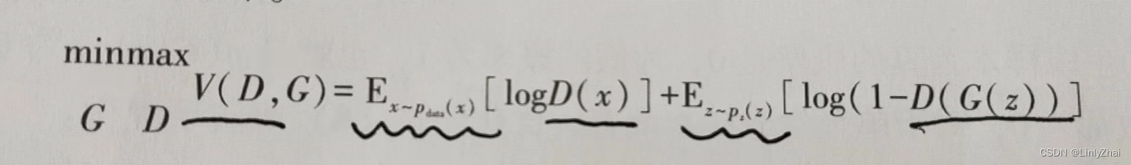
1.1损失函数

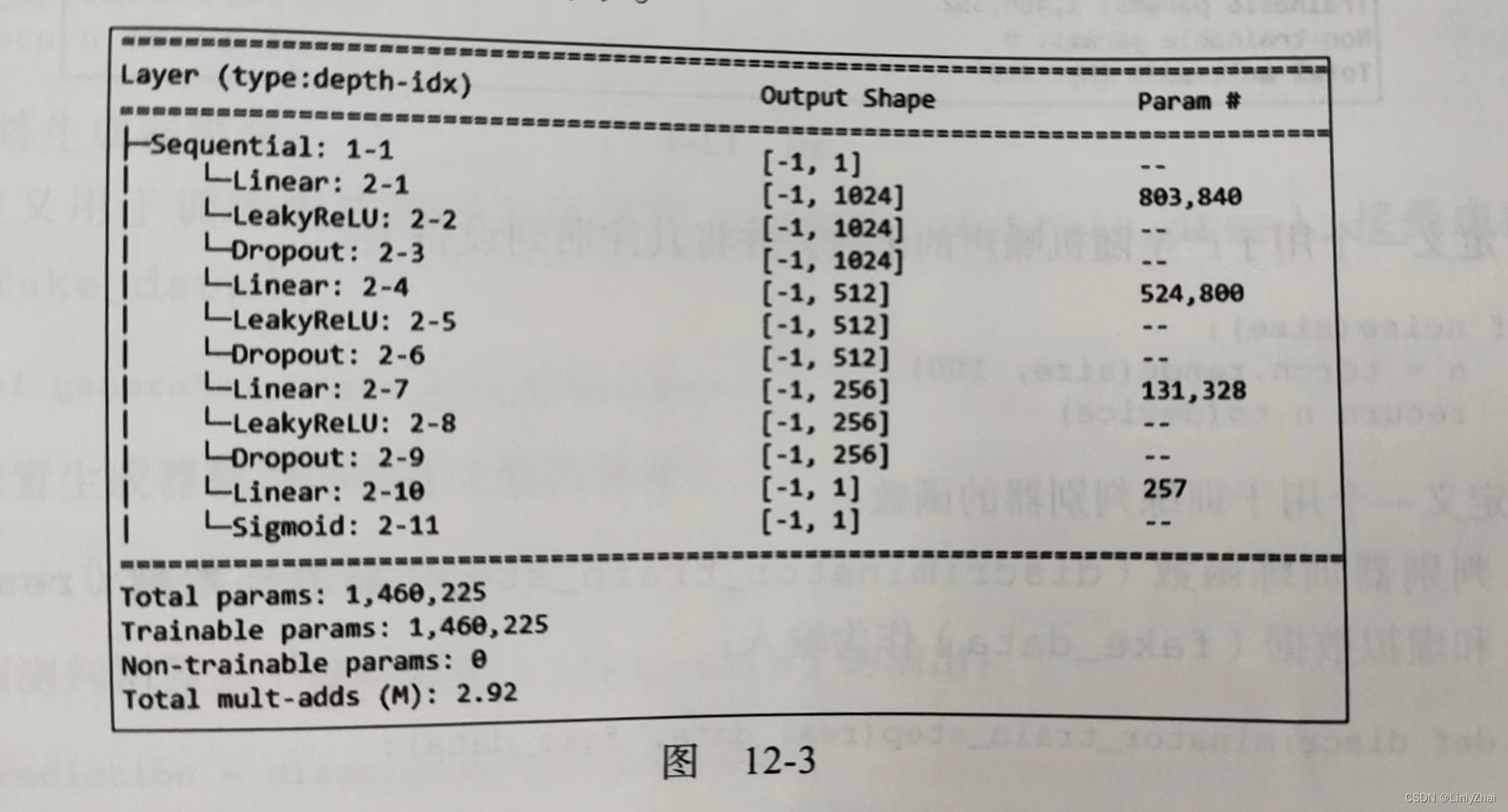
1.2判别器源码

class Discriminator(nn.Module):
	def __init__(self):
		super().__init__()
		self.model = nn.Sequential(
						nn.Linear(784,1024),
						nn.LeakyReLU(0.2),
						nn.Dropout(0.3),
						nn.Linear(1024,512),
						nn.LeakyReLU(0.2),
						nn.Dropout(0.3),
						nn.Linear(512,256),
						nn.LeakyReLU(0.2),
						nn.Dropout(0.3),
						nn.Linear(256,1),
						nn.Sigmoid()
 		)
 	def forward(self, x):
 		return self.model(x)

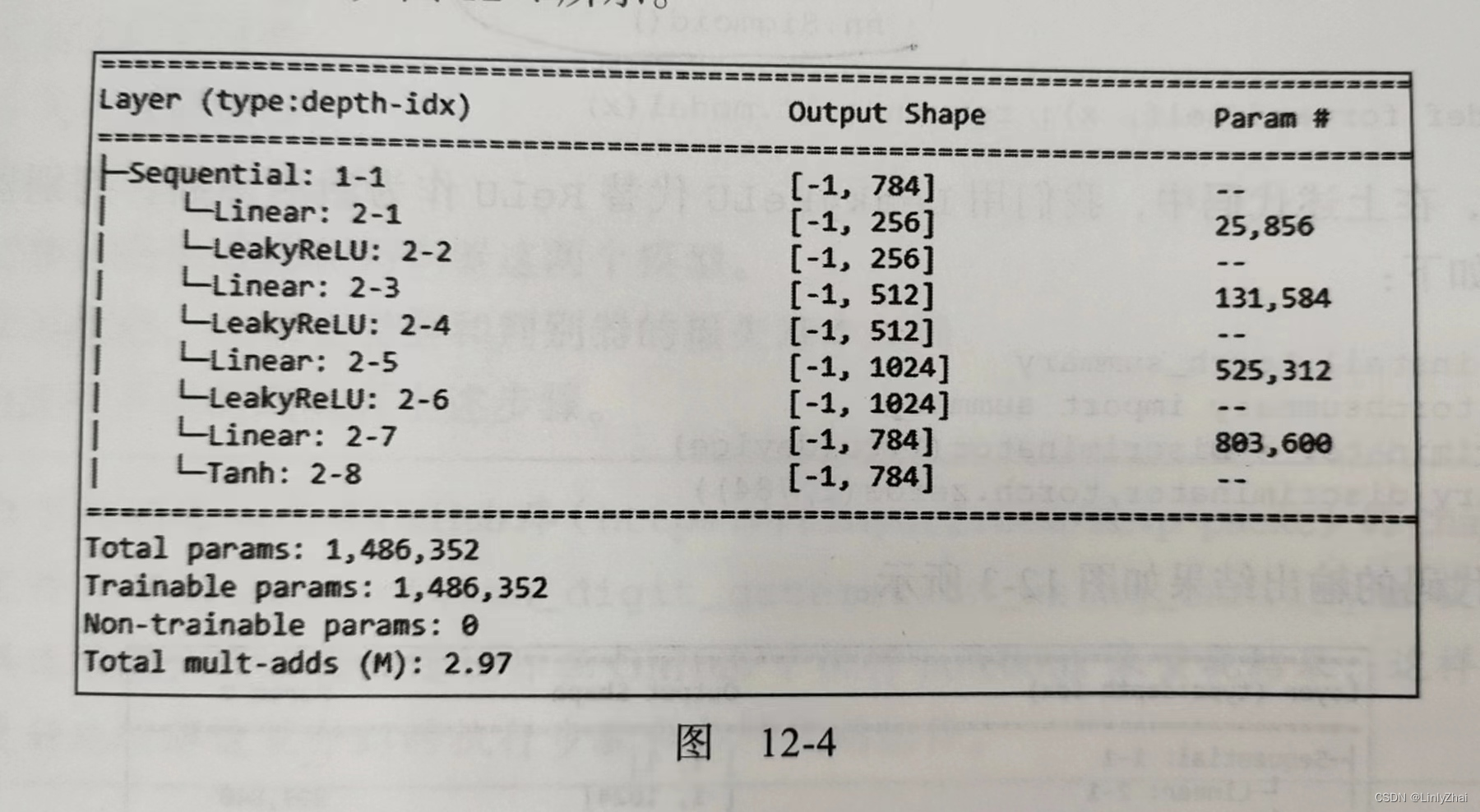
1.3 生成器源码

class Generator(nn.Module):
	def __init__(self):
		super().__init__()
		self.model = nn.Sequential(
						nn.Linear(100,256),
						nn.LeakyReLU(0.2),
						
						nn.Linear(256,512),
						nn.LeakyReLU(0.2),
						
						nn.Linear(512,1024),
						nn.LeakyReLU(0.2),
					
						nn.Linear(1024,784),
						nn.Tahn()
 		)
 	def forward(self, x):
 		return self.model(x)

二、什么是CGAN？

CGAN,全称Conditional Generative Aderversarial Networks.与GAN相比，条件GAN加入了额外信息c，从而能够生成指定的手写数字。

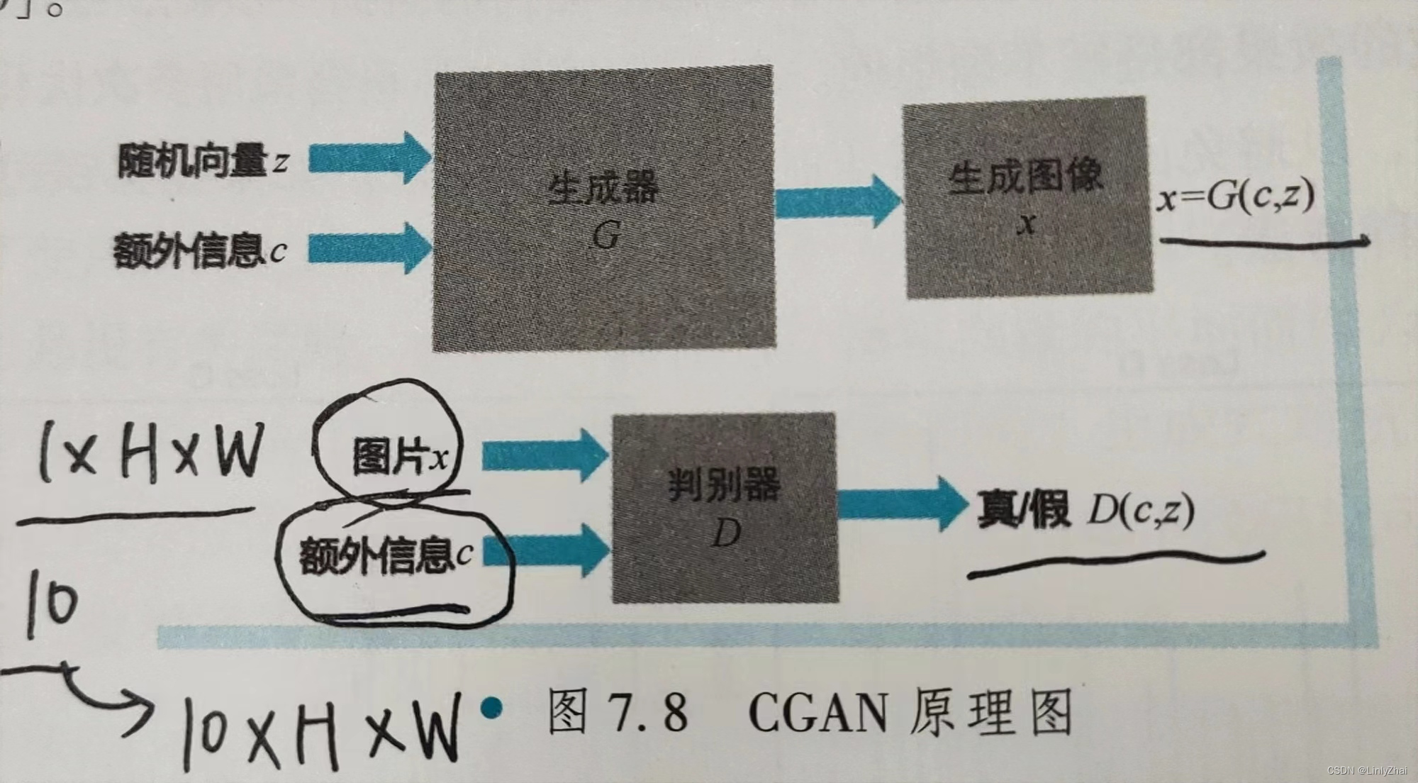
2.1 CGAN原理图

2.2条件GAN的损失函数

nn.BCELoss()是一个PyTorch中的损失函数，它被用于二分类问题。BCE代表二元交叉熵（Binary Cross Entropy）
这里用到的是二元交叉熵损失函数
D(x)代表的是判别器判别图片是真的概率；
在

2.3 生成器源码

class Generator(nn.Module):
    def __init__(self, num_channel=1, nz=100, nc=10, ngf=64):
        super(Generator, self).__init__()
        self.main = nn.Sequential(
            # 输入维度 110 x 1 x 1
            nn.ConvTranspose2d(nz + nc, ngf * 8, 4, 1, 0, bias=False),
            nn.BatchNorm2d(ngf * 8),
            nn.ReLU(True),
            # 特征维度 (ngf*8) x 4 x 4
            nn.ConvTranspose2d(ngf * 8, ngf * 4, 4, 2, 1, bias=False),
            nn.BatchNorm2d(ngf * 4),
            nn.ReLU(True),
            # 特征维度 (ngf*4) x 8 x 8
            nn.ConvTranspose2d(ngf * 4, ngf * 2, 4, 2, 1, bias=False),
            nn.BatchNorm2d(ngf * 2),
            nn.ReLU(True),
            # 特征维度 (ngf*2) x 16 x 16
            nn.ConvTranspose2d(ngf * 2, ngf, 4, 2, 1, bias=False),
            nn.BatchNorm2d(ngf),
            nn.ReLU(True),
            # 特征维度 (ngf) x 32 x 32
            nn.ConvTranspose2d(ngf, num_channel, 4, 2, 1, bias=False),
            nn.Tanh()
            # 特征维度. (num_channel) x 64 x 64
        )
        self.apply(weights_init)

    def forward(self, input_z, onehot_label):
        input_ = torch.cat((input_z, onehot_label), dim=1)
        n, c = input_.size()
        input_ = input_.view(n, c, 1, 1)
        return self.main(input_)

在生成器，
随机向量z是100维的，
额外信息c是10维的，（因为手写数字包含0-9，一共10类）
在这里，采用直接拼接的方式，最终形成了110维的输入

2.4 判别器源码

class Discriminator(nn.Module):
    def __init__(self, num_channel=1, nc=10, ndf=64):
        super(Discriminator, self).__init__()
        self.main = nn.Sequential(
            # 输入维度 (num_c3
            # channel+nc) x 64 x 64  1*64*64的图像和10维的类别   10维类别先转换成10*64*64    然后合并就是11*64*64
            # 输入通道  输出通道   卷积核的大小   步长  填充
            #原始输入张量：b 11 64  64
            nn.Conv2d(num_channel + nc, ndf, 4, 2, 1, bias=False),   #b  64  32  32
            nn.LeakyReLU(0.2, inplace=True),
            # 特征维度 (ndf) x 32 x 32
            nn.Conv2d(ndf, ndf * 2, 4, 2, 1, bias=False),  #b   64*2   16  16
            nn.BatchNorm2d(ndf * 2),
            nn.LeakyReLU(0.2, inplace=True),
            # 特征维度 (ndf*2) x 16 x 16
            nn.Conv2d(ndf * 2, ndf * 4, 4, 2, 1, bias=False),    #b   64*4   8    8
            nn.BatchNorm2d(ndf * 4),
            nn.LeakyReLU(0.2, inplace=True),
            # 特征维度 (ndf*4) x 8 x 8
            nn.Conv2d(ndf * 4, ndf * 8, 4, 2, 1, bias=False),    #b   64*8    4    4
            nn.BatchNorm2d(ndf * 8),
            nn.LeakyReLU(0.2, inplace=True),
            # 特征维度 (ndf*8) x 4 x 4
            nn.Conv2d(ndf * 8, 1, 4, 1, 0, bias=False),        #b   1    1    1      其实就是一个数值，区间在正无穷到负无穷之间
            nn.Sigmoid()
        )
        self.apply(weights_init)

    def forward(self, images, onehot_label):
        device = 'cuda' if torch.cuda.is_available() else 'cpu'
        h, w = images.shape[2:]
        n, nc = onehot_label.shape[:2]
        label = onehot_label.view(n, nc, 1, 1) * torch.ones([n, nc, h, w]).to(device)
        input_ = torch.cat([images, label], 1)
        return self.main(input_)

在判别器中，输入的数据有
图片x,(可能是来自真实数据集的样本，也可能是来自生成器生成的虚假样本) 维度是1 * H * W
额外信息c，维度是10维，变换到10 * 1 * 1，将后两维进行复制 变换为10 * H * W的张量；
最终拼接在一起，构成11 * H * W的输入。

2.5 训练过程

MODEL_G_PATH = "./"
LOG_G_PATH = "Log_G.txt"
LOG_D_PATH = "Log_D.txt"
IMAGE_SIZE = 64
BATCH_SIZE = 128
WORKER = 1
LR = 0.0002
NZ = 100
NUM_CLASS = 10
EPOCH = 50

data_loader = loadMNIST(img_size=IMAGE_SIZE, batch_size=BATCH_SIZE)  #原始图片宽高是28*28的，给改变成64*64
device = torch.device("cuda:0" if torch.cuda.is_available() else "cpu")
netG = Generator().to(device)
netD = Discriminator().to(device)
criterion = nn.BCELoss()
real_label = 1.
fake_label = 0.
optimizerD = optim.Adam(netD.parameters(), lr=LR, betas=(0.5, 0.999))
optimizerG = optim.Adam(netG.parameters(), lr=LR, betas=(0.5, 0.999))

g_writer = LossWriter(save_path=LOG_G_PATH)
d_writer = LossWriter(save_path=LOG_D_PATH)

fix_noise = torch.randn(BATCH_SIZE, NZ, device=device)
fix_input_c = (torch.rand(BATCH_SIZE, 1) * NUM_CLASS).type(torch.LongTensor).squeeze().to(device)
fix_input_c = onehot(fix_input_c, NUM_CLASS)

img_list = []
G_losses = []
D_losses = []
iters = 0

print("开始训练>>>")
for epoch in range(EPOCH):

    print("正在保存网络并评估...")
    save_network(MODEL_G_PATH, netG, epoch)
    with torch.no_grad():
        fake_imgs = netG(fix_noise, fix_input_c).detach().cpu()
        images = recover_image(fake_imgs)
        full_image = np.full((5 * 64, 5 * 64, 3), 0, dtype="uint8")
        for i in range(25):
            row = i // 5
            col = i % 5
            full_image[row * 64:(row + 1) * 64, col * 64:(col + 1) * 64, :] = images[i]
            # ！！！！！！！！！！！！！！
            #每一轮次结束后，这里只展示了一批图片的前25张。
        plt.imshow(full_image)
        #plt.show()
        plt.imsave("{}.png".format(epoch), full_image)

    for data in data_loader:
       
        netD.zero_grad()
        real_imgs, input_c = data   #这里的input_c其实就是数据集每一批中的每个图片对应的标签
        input_c = input_c.to(device)
        input_c = onehot(input_c, NUM_CLASS).to(device)

        # 1.1 来自数据集的样本
        real_imgs = real_imgs.to(device)
        b_size = real_imgs.size(0)
        label = torch.full((b_size,), real_label, dtype=torch.float, device=device)
        #上面的torch.full是生成一维的 b_size这么多的，填充值为1.的张量
        # real_label = 1.
        # fake_label = 0.

        # 使用判别器对真实数据集样本做判断
        #！！！！！！！！！！！！！
        #output应该是判别器判别一批真图片真实的概率
        output = netD(real_imgs, input_c).view(-1)   
        errD_real = criterion(output, label)
        #！！！！！！
        #errD_real是判别器识别真图片的误差，为了训练判别器判别真图片为真
        errD_real.backward()
        D_x = output.mean().item()   
        #！！！！！！！
        #D_x就是判别器判别一批真图片为真的概率的平均值

        
        # 1.2 生成随机向量   这一步想要训练判别器是否能够识别出是虚假图片
        noise = torch.randn(b_size, NZ, device=device)
        # 生成随机标签
        input_c = (torch.rand(b_size, 1) * NUM_CLASS).type(torch.LongTensor).squeeze().to(device)
        input_c = onehot(input_c, NUM_CLASS)

        # 来自生成器生成的样本
        fake = netG(noise, input_c)
        label.fill_(fake_label)

        # real_label = 1.
        # fake_label = 0.
        # 使用判别器对生成器生成样本做判断
        #！！！！！！！！！！！
        #output应该是判别器判别一批假图片真实的概率
        output = netD(fake.detach(), input_c).view(-1)  
        errD_fake = criterion(output, label)
        # 对判别器进行梯度回传
        errD_fake.backward()
        #！！！！！！
        #errD_fake是判别器识别假图片的误差，为了训练判别器判别假图片为假
        D_G_z1 = output.mean().item()
        #！！！！！！！！！！！！
        #D_G_z1就是判别器判别一批假图片为真的概率的平均值
        errD = errD_real + errD_fake
        #！！！！！！
        #errD是判别器识别真实图片和假图片的误差和
        # 更新判别器
        optimizerD.step()


        
       
        netG.zero_grad()
        # 对于生成器训练，令生成器生成的样本为真，
        label.fill_(real_label)

        # real_label = 1.
        # fake_label = 0.
        #！！！！！！！！！！！
        #output应该是判别器判别一批假图片真实的概率
        output = netD(fake, input_c).view(-1)
        # 对生成器计算损失
        errG = criterion(output, label)
         #！！！！！！
        #errG是判别器识别假图片的误差,但是是为了训练生成器生成假图片，以假乱真
        # 因为这里判别器的角度label真实应该是0，但是站在生成器的角度，label真实应该是1，即生成器希望生成的虚假图片让判别器识别的时候，会误以为1才比较好，即误以为是真实的图片
        # 所以生成器交叉熵也是越小越好
        # 对生成器进行梯度回传
        errG.backward()
        D_G_z2 = output.mean().item()
        #！！！！！！！！！！！！
        #D_G_z2就是判别器判别一批假图片为真的概率的平均值
        # 更新生成器
        optimizerG.step()

        # 输出损失状态
        if iters % 5 == 0:
            print('[%d/%d][%d/%d]\tLoss_D: %.4f\tLoss_G: %.4f\tD(x): %.4f\tD(G(z)): %.4f / %.4f'
                  % (epoch, EPOCH, iters % len(data_loader), len(data_loader),
                     errD.item(), errG.item(), D_x, D_G_z1, D_G_z2))
            d_writer.add(loss=errD.item(), i=iters)
            g_writer.add(loss=errG.item(), i=iters)

        # 保存损失记录
        G_losses.append(errG.item())
        D_losses.append(errD.item())

        iters += 1

1）这里的训练顺序

这里训练的顺序是
先拿真实图片训练判别器，
再拿假图片训练判别器，
最后，拿假图片让判别器判断，来训练生成器。

2）为什么先训练判别器后训练生成器呢？

试想，假如先训练生成器，但是刚开始判别器还没有判别能力，所以达不到训练生成器，帮助生成器能越来越生成逼真的假图片。
所以，需要先训练判别器，让判别器先具有初步的判别能力，才能训练生成器，帮助生成器能够生成逼真的假图片。

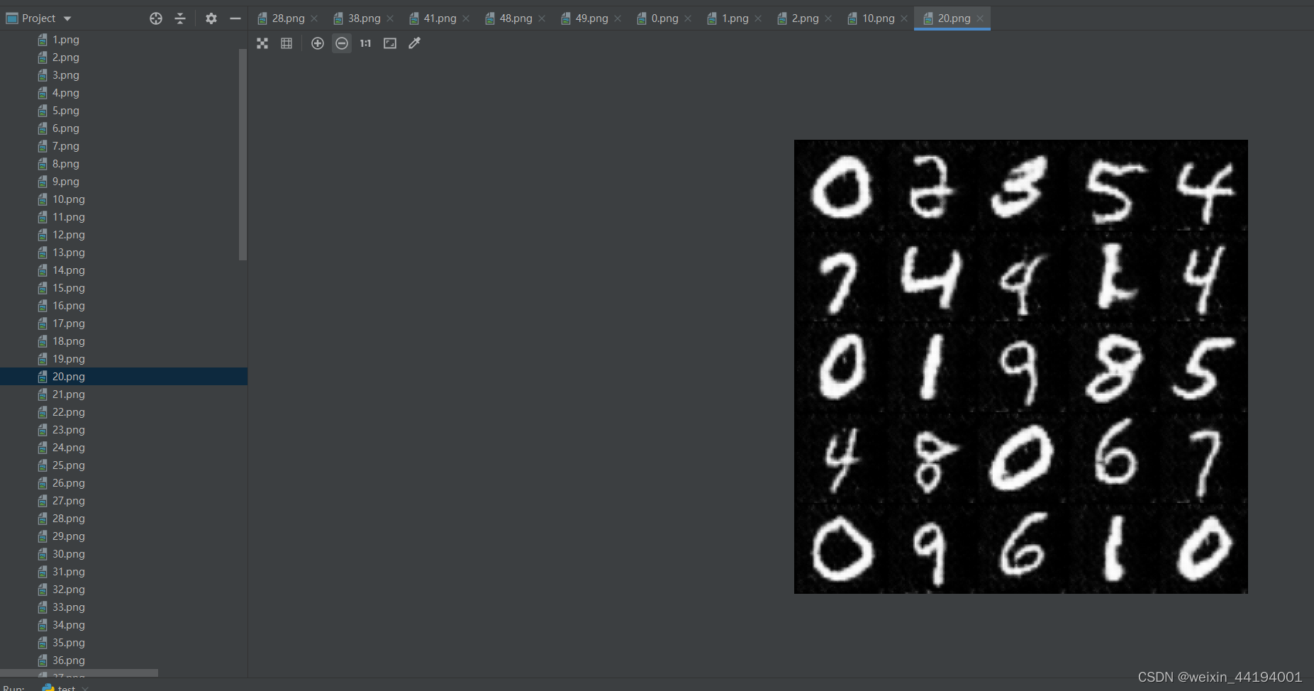
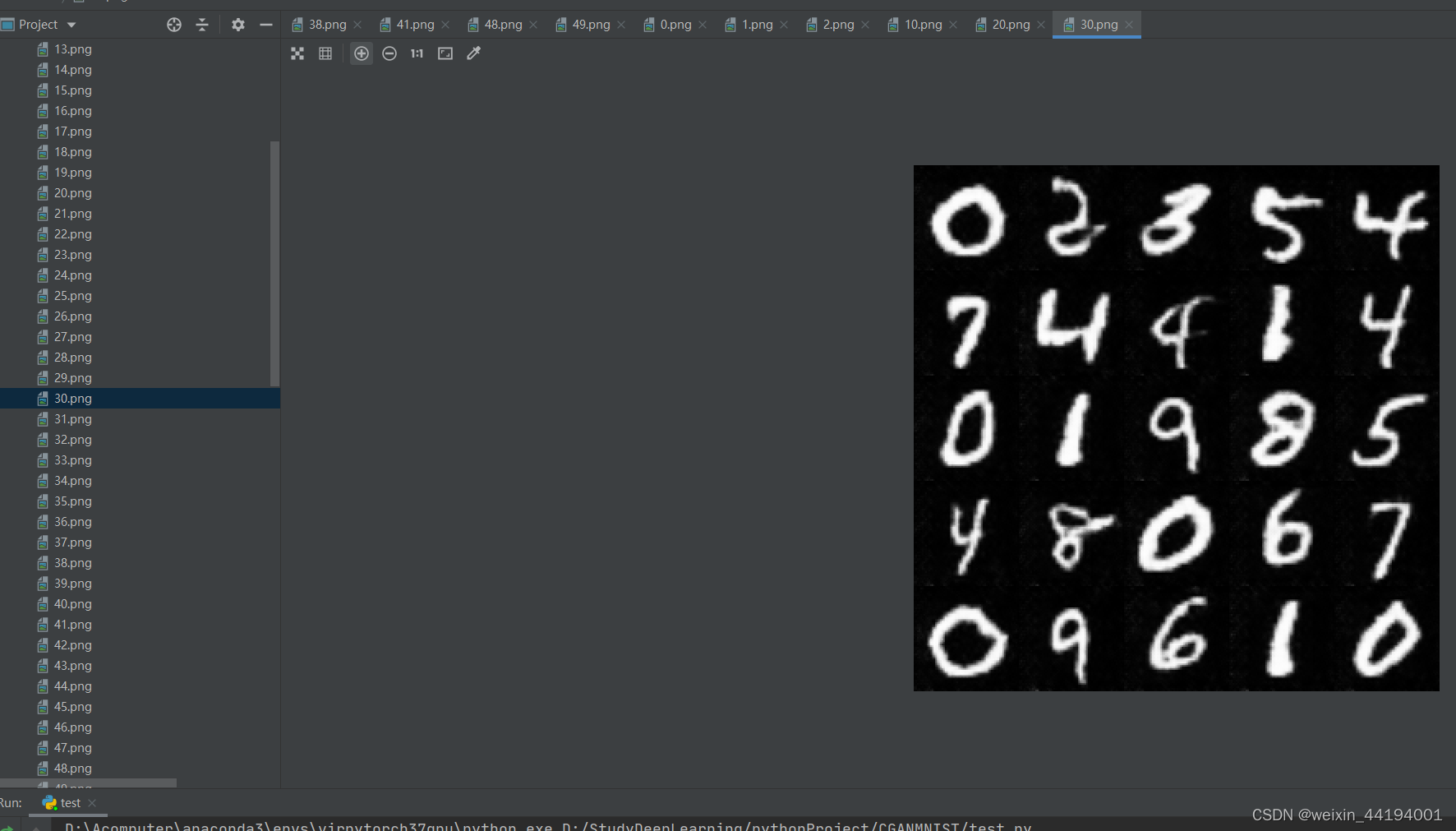
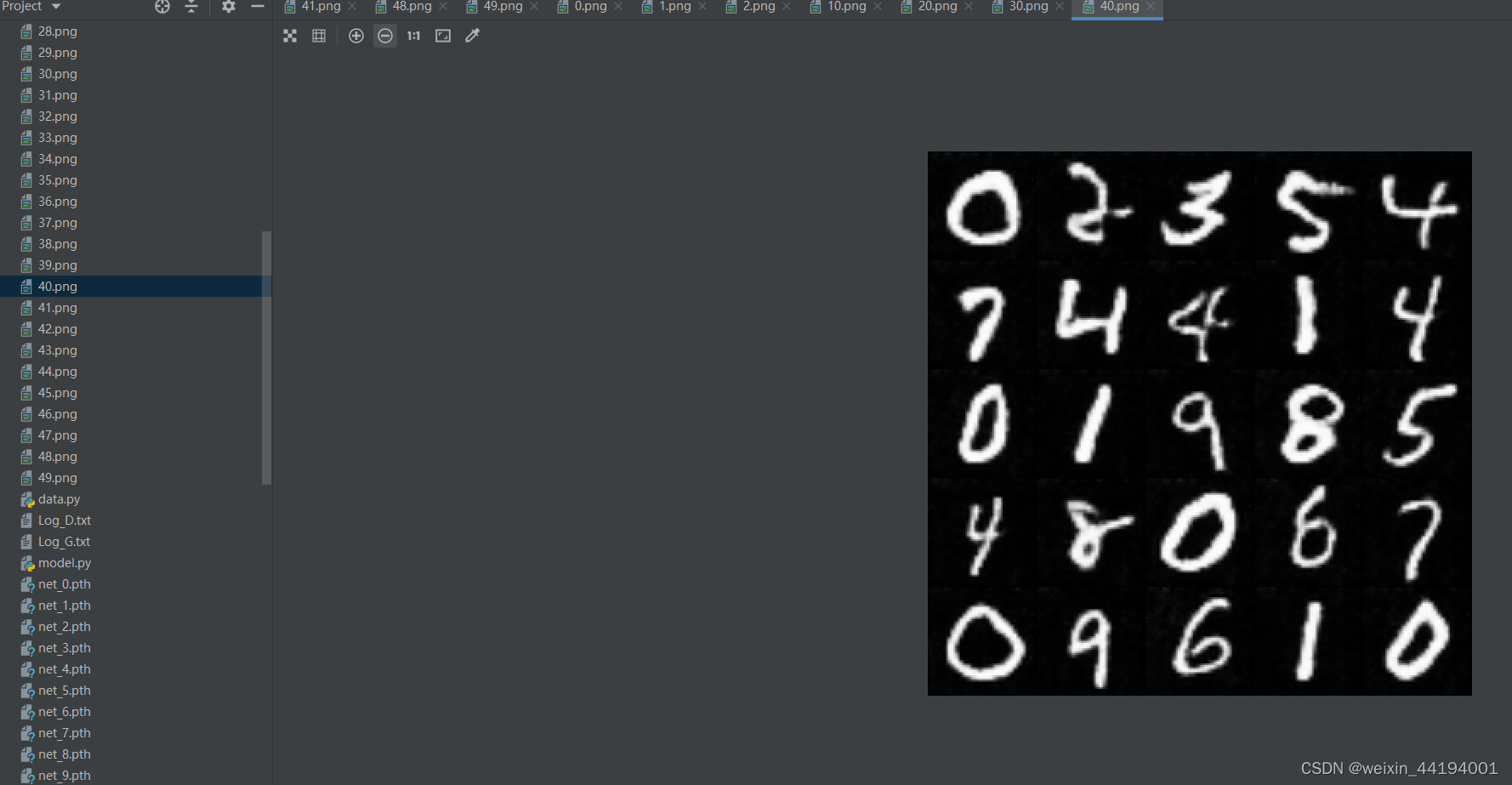
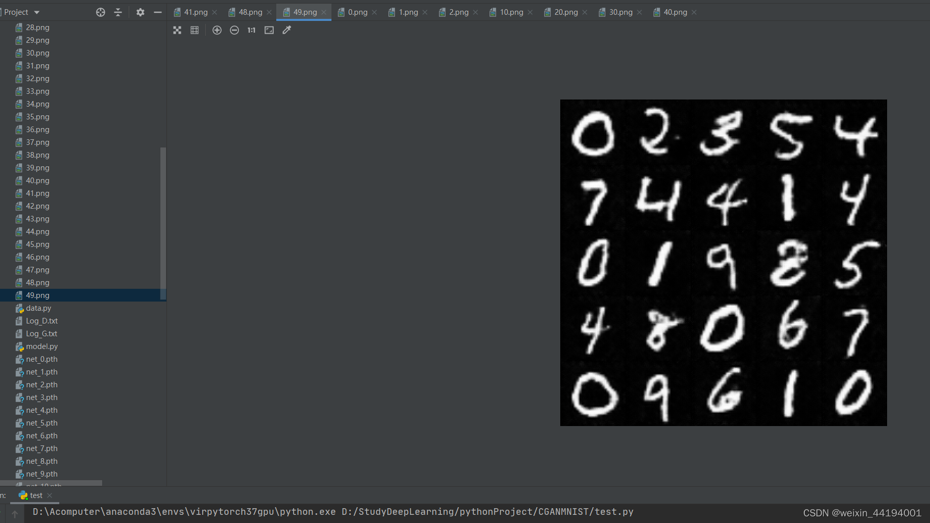
2.6 训练过程运行结果

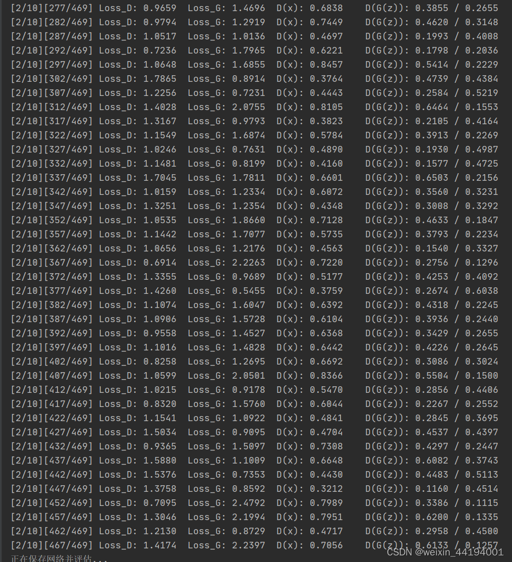
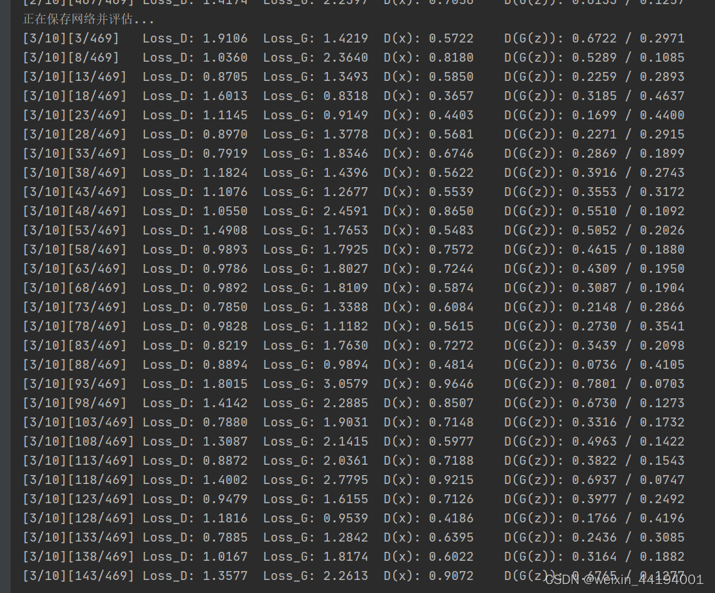
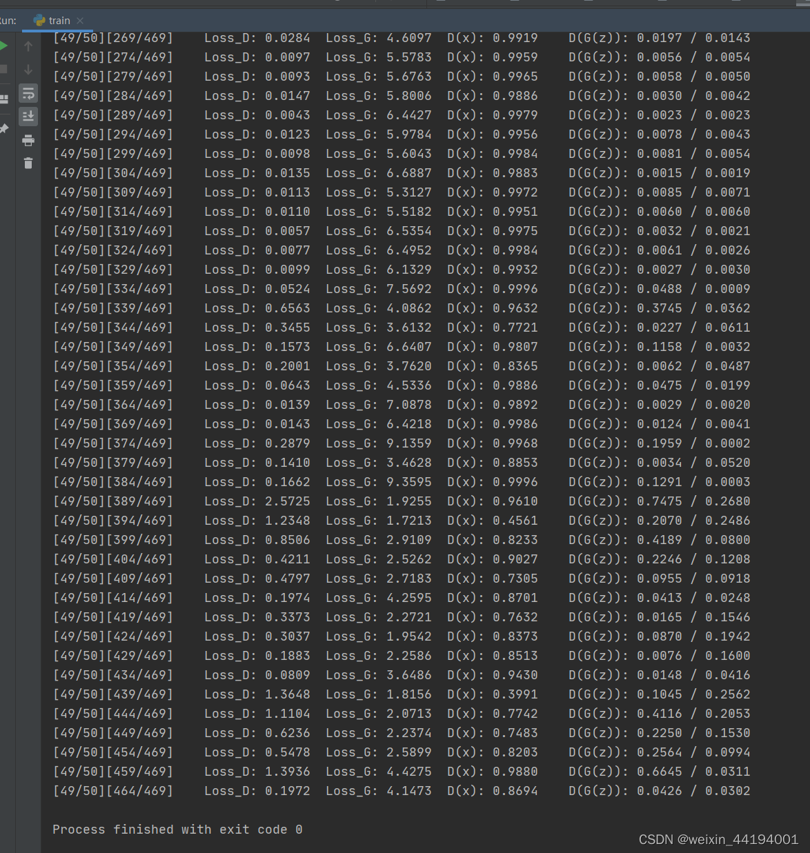
#errD是判别器识别真实图片和假图片的误差和，是为了训练判别器能够判别真假图片
#errG是判别器识别假图片的误差,但是是为了训练生成器生成假图片，以假乱真
#D_x就是判别器判别一批真图片为真的概率的平均值，训练判别器识别真图片
#D_G_z1就是判别器判别一批假图片为真的概率的平均值，训练判别器识别假图片
#D_G_z2就是判别器判别一批假图片为真的概率的平均值，训练生成器生成逼真的假图片

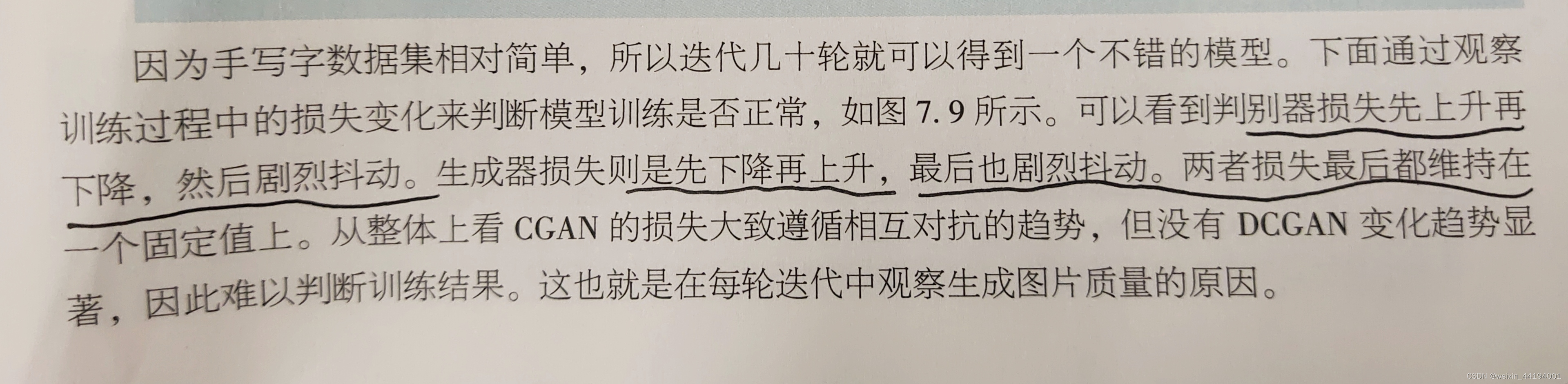
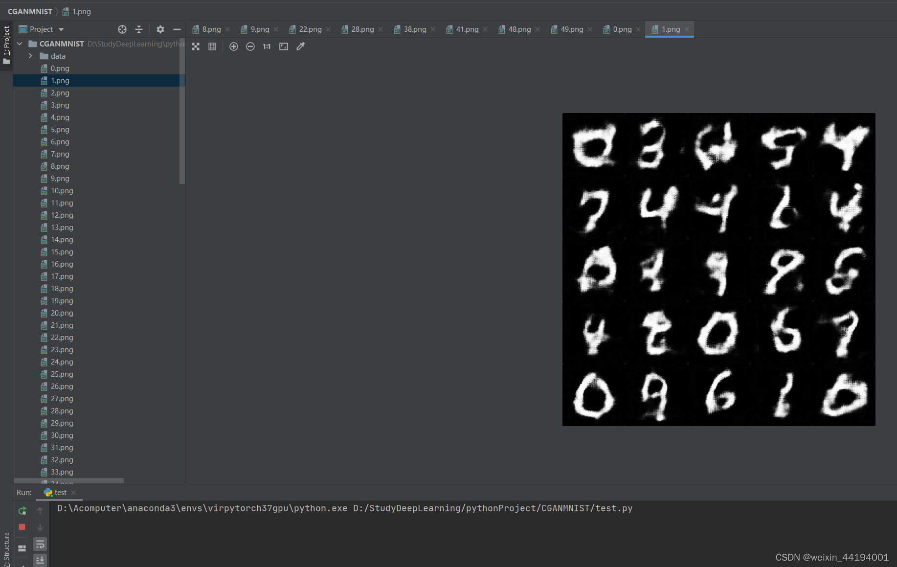
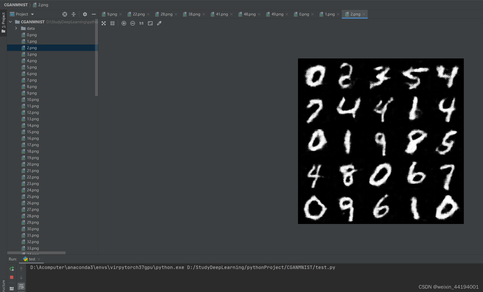
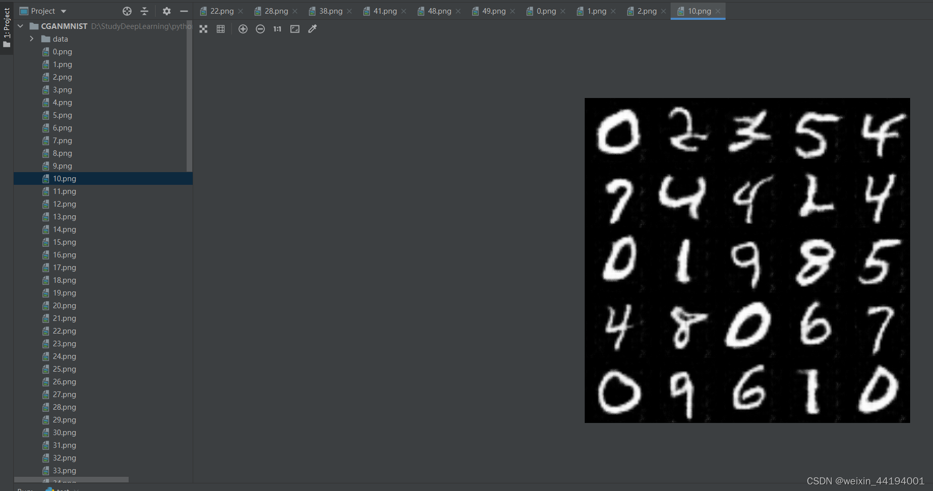
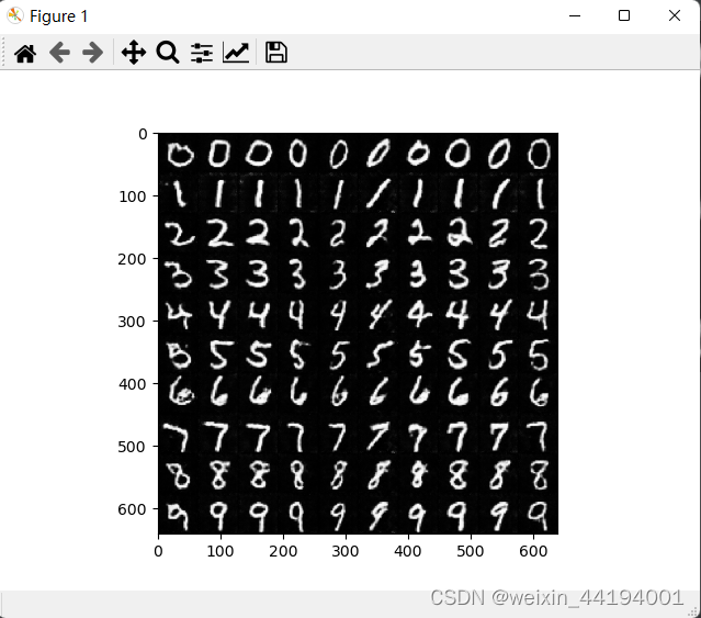
2.7测试结果

1)测试代码

NZ = 100
NUM_CLASS = 10
BATCH_SIZE = 10
DEVICE = "cpu"

netG = Generator()
netG = restore_network("./", "49", netG)
fix_noise = torch.randn(BATCH_SIZE, NZ, device=DEVICE)
fix_input_c = torch.tensor([0, 0, 0, 0, 0, 0, 0, 0, 0, 0])
device = "cuda" if torch.cuda.is_available() else "cpu"
fix_input_c = onehot(fix_input_c, NUM_CLASS)
fix_input_c = fix_input_c.to(device)
fix_noise = fix_noise.to(device)
netG = netG.to(device)
#fake_imgs = netG(fix_noise, fix_input_c).detach().cpu()



#fix_noise = torch.randn(BATCH_SIZE, NZ, device=DEVICE)
full_image = np.full((10 * 64, 10 * 64, 3), 0, dtype="uint8")
for num in range(10):
    input_c = torch.tensor(np.ones(10, dtype="int64") * num)
    input_c = onehot(input_c, NUM_CLASS)
    fix_noise = fix_noise.to(device)
    input_c = input_c.to(device)
    fake_imgs = netG(fix_noise, input_c).detach().cpu()
    images = recover_image(fake_imgs)
    for i in range(10):
        row = num
        col = i % 10
        full_image[row * 64:(row + 1) * 64, col * 64:(col + 1) * 64, :] = images[i]

plt.imshow(full_image)
plt.show()
plt.imsave("hah.png", full_image)